Object tracking using a Kalman filter (MATLAB)

The Kalman filter is useful for tracking different types of moving objects. It was originally invented by Rudolf Kalman at NASA to track the trajectory of spacecraft. At its heart, the Kalman filter is a method of combining noisy (and possibly missing) measurements and predictions of the state of an object to achieve an estimate of its true current state. Kalman filters can be applied to many different types of linear dynamical systems and the “state” here can refer to any measurable quantity, such as an object’s location, velocity, temperature, voltage, or a combination of these.

In a previous article, I showed how face detection can be performed in MATLAB using OpenCV. In this article, I will combine this face detector with a Kalman filter to build a simple face tracker that can track a face in a video.

If you are unfamiliar with Kalman filters, I suggest you read up first on how alpha beta filters work. They are a simplified version of the Kalman filter that are much easier to understand, but still apply many of the core ideas of the Kalman filter.

Face tracking without a Kalman filter

The OpenCV-based face detector can be applied to every frame to detect the location of the face. Because it may detect multiple faces, we need a method to find the relationship between a detected face in one frame to another face in the next frame — this is a combinatorial problem known as data association. The simplest method is the nearest neighbour approach, and some other methods can be found in this survey paper on object tracking. However, to greatly simplify the problem, the tracker I have implemented is a single face tracker and it assumes there is always a face in the frame. This means that every face that is detected can be assumed to be the same person’s face. If more than one face is detected, only the first face is used. If no faces are detected, a detection error is assumed. The MATLAB code below will detect the face location in a sequence of images and output the bounding box coordinates to a CSV file.

function detect_faces(imgDir, opencvPath, includePath, outputFilename)

    % Load the required libraries

    if libisloaded('highgui100'), unloadlibrary highgui100, end
    if libisloaded('cv100'), unloadlibrary cv100, end
    if libisloaded('cxcore100'), unloadlibrary cxcore100, end

    loadlibrary(...
        fullfile(opencvPath, 'bin\cxcore100.dll'), @proto_cxcore);
    loadlibrary(...
        fullfile(opencvPath, 'bin\cv100.dll'), ...
        fullfile(opencvPath, 'cv\include\cv.h'), ...
            'alias', 'cv100', 'includepath', includePath);
    loadlibrary(...
        fullfile(opencvPath, 'bin\highgui100.dll'), ...
        fullfile(opencvPath, 'otherlibs\highgui\highgui.h'), ...
            'alias', 'highgui100', 'includepath', includePath);

    % Load the cascade

    classifierFilename = 'C:/Program Files/OpenCV/data/haarcascades/haarcascade_frontalface_alt.xml';
    cvCascade = calllib('cv100', 'cvLoadHaarClassifierCascade', classifierFilename, libstruct('CvSize',struct('width',int16(100),'height',int16(100))));

    % Create memory storage

    cvStorage = calllib('cxcore100', 'cvCreateMemStorage', 0);

    % Get the list of images
    imageFiles = dir(imgDir);
    detections = struct;

    h = waitbar(0, 'Performing face detection...'); % progress bar

    % Open the output CSV file
    fid = fopen(outputFilename, 'w');
    fprintf(fid, 'filename,x1,y1,x2,y2');

    for i = 1:numel(imageFiles)

        if imageFiles(i).isdir; continue; end
        imageFile = fullfile(imgDir, imageFiles(i).name);

        % Load the input image
        cvImage = calllib('highgui100', ...
            'cvLoadImage', imageFile, int16(1));
        if ~cvImage.Value.nSize
            error('Image could not be loaded');
        end

        % Perform face detection
        cvSeq = calllib('cv100', 'cvHaarDetectObjects', cvImage, cvCascade, cvStorage, 1.1, 2, 0, libstruct('CvSize',struct('width',int16(40),'height',int16(40))));

        % Save the detected bounding box, if any (and if there's multiple
        % detections, just use the first one)
        detections(i).filename = imageFile;
        if cvSeq.Value.total == 1
            cvRect = calllib('cxcore100', ...
                'cvGetSeqElem', cvSeq, int16(1));
            fprintf(fid, '%s,%d,%d,%d,%d', imageFile, ...
                cvRect.Value.x, cvRect.Value.y, ...
                cvRect.Value.x + cvRect.Value.width, ...
                cvRect.Value.y + cvRect.Value.height);
        else
            fprintf(fid, '%s,%d,%d,%d,%d', imageFile, 0, 0, 0, 0);
        end

        % Release image
        calllib('cxcore100', 'cvReleaseImage', cvImage);
        waitbar(i / numel(imageFiles), h);

    end

    % Release resources

    fclose(fid);
    close(h);
    calllib('cxcore100', 'cvReleaseMemStorage', cvStorage);
    calllib('cv100', 'cvReleaseHaarClassifierCascade', cvCascade);

end

We can then run our face detector and generate an output file, faces.csv, like this:

imgDir = 'images';
opencvPath = 'C:\Program Files\OpenCV';
includePath = fullfile(opencvPath, 'cxcore\include');
detect_faces(imgDir, opencvPath, includePath, 'faces.csv');

In the video below, I have run this script on the FGnet Talking Face database (which is free to download) and displayed the bounding boxes overlayed on the image sequence. You can download a copy of the faces.csv file that was used to generate the video from here.

The bounding box roughly follows the face, but its trajectory is quite noisy and the video contains numerous frames where the bounding box disappears because the face was not detected. The Kalman filter can be used to smooth this trajectory and estimate the location of the bounding box when the face detector fails.

Kalman filtering: The gritty details

The Kalman filter is a recursive two-stage filter. At each iteration, it performs a predict step and an update step.

The predict step predicts the current location of the moving object based on previous observations. For instance, if an object is moving with constant acceleration, we can predict its current location, , based on its previous location, , using the equations of motion.

The update step takes the measurement of the object’s current location (if available), , and combines this with the predicted current location, , to obtain an a posteriori estimated current location of the object, .

The equations that govern the Kalman filter are given below (taken from the Wikipedia article):

1. Predict stage:
   1. Predicted (a priori) state:
   2. Predicted (a priori) estimate covariance:
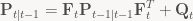
2. Update stage:
   1. Innovation or measurement residual:
   2. Innovation (or residual) covariance:
   3. Optimal Kalman gain:
   4. Updated (a posteriori) state estimate:
   5. Updated (a posteriori) estimate covariance:

They can be difficult to understand at first, so let’s first take a look at what each of these variables are used for:

• is the current state vector, as estimated by the Kalman filter, at time .
• is the measurement vector taken at time .
• measures the estimated accuracy of at time .
• describes how the system moves (ideally) from one state to the next, i.e. how one state vector is projected to the next, assuming no noise (e.g. no acceleration)
• defines the mapping from the state vector, , to the measurement vector, .
• and define the Gaussian process and measurement noise, respectively, and characterise the variance of the system.
• and are control-input parameters are only used in systems that have an input; these can be ignored in the case of an object tracker.

Note that in a simple system, the current state and the measurement will contain the same set of state variables (only will be a filtered version of ) and will be an identity matrix, but many real-world systems will include latent variables that are not directly measured. For example, if we are tracking the location of a car, we may be able to directly measure its location from a GPS device and its velocity from the speedometer, but not its acceleration.

In the predict stage, the state of the system and its error covariance are transitioned using the defined transition matrix , and can be implemented in MATLAB as:

function [x,P] = kalman_predict(x,P,F,Q)
    x = F*x; %predicted state
    P = F*P*F' + Q; %predicted estimate covariance
end

In the update stage, we first calculate the difference between our predicted and measured states. We then calculate the Kalman gain matrix, , which is used to weight between our predicted and measured states and is adjusted based on a ratio of prediction error to measurement noise .

Finally, the state vector and its error covariance are then updated with the measured state. It can be implemented in MATLAB as:

function [x,P] = kalman_update(x,P,z,H,R)
    y = z - H*x; %measurement error/innovation
    S = H*P*H' + R; %measurement error/innovation covariance
    K = P*H'*inv(S); %optimal Kalman gain
    x = x + K*y; %updated state estimate
    P = (eye(size(x,1)) - K*H)*P; %updated estimate covariance
end

Both the stages only update two variables: , the state variable, and , the prediction error covariance variable.

The two stages of the filter correspond to the state-space model typically used to model linear dynamical systems. The first stage solves the process equation:

The process noise is additive Gaussian white noise (AWGN)with zero mean and covariance defined by:

The second one is the measurement equation:

The measurement noise is also AGWN with zero mean and covariance defined by:

Defining the system

In order to implement a Kalman filter, we have to define several variables that model the system. We have to choose the variables contained by and , and also choose suitable values for , , and , as well as an initial value for .

We will define our measurement vector as:

where and are the upper-left and lower-right corners of the bounding box around the detected face, respectively. This is simply the output from the Viola and Jones face detector.

A logical choice for our state vector is:

where and are the first-order derivatives. Other vectors are also possible; for example, some papers introduce a “scale” variable, which assumes that the bounding box maintains a fixed aspect ratio.

The transition matrix defines the equations used to transition from one state vector to the next vector (without taking into account any measurements, ). It is plugged in to the process equation:

Let’s look at some basic equations describing motion:

We could express this system using the following recurrence:

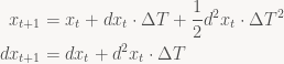
These same equations can also be used to model the variables and their derivatives. Referring back to the process equation, we can thus model this system as:

The process noise matrix measures the variability of the input signal away from the “ideal” transitions defined in the transition matrix. Larger values in this matrix mean that the input signal has greater variance and the filter needs to be more adaptable. Smaller values result in a smoother output, but the filter is not as adaptable to large changes. This can be a little difficult to define, and may require some fine tuning. Based on our definition of the measurement noise above, our process noise matrix is defined as:

where and .

The measurement matrix maps between our measurement vector and state vector . It is plugged in to the measurement equation:

The variables and are mapped directly from to , whereas the derivative variables are latent (hidden) variables and so are not directly measured and are not included in the mapping. This gives us the measurement matrix:

The matrix defines the error of the measuring device. For a physical instrument such as a speedometer or voltmeter, the measurement accuracy may be defined by the manufacturer. In the case of a face detector, we can determine the accuracy empirically. For instance, we may find that our Viola and Jones face detector detects faces to within 10 pixels of the actual face location 95% of the time. If we assume this error is Gaussian-distributed (which is a requirement of the Kalman filter), this gives us a variance of 6.5 pixels for each of the coordinates, so the measurement noise vector is then given by:

The errors are independent, so our covariance matrix is given by:

Decreasing the values in means we are optimistically assuming our measurements are more accurate, so the filter performs less smoothing and the predicted signal will follow the observed signal more closely. Conversely, increasing means we have less confidence in the accuracy of the measurements, so more smoothing is performed.

The estimate covariance matrix is a measure of the estimated accuracy of at time . It is adjusted over time by the filter, so we only need to supply a reasonable initial value. If we know for certain the exact state variable at start-up, then we can initialise to a matrix of all zeros. Otherwise, it should be initialised as a diagonal matrix with a large value along the diagonal:

where . The filter will then prefer the information from the first few measurements over the information already in the model.

Implementing the face tracker

The following script implements the system we have defined above. It loads the face detection results from CSV file, performs the Kalman filtering, and displays the detected bounding boxes.

% read in the detected face locations
fid = fopen('detect_faces.csv');
fgetl(fid); %ignore the header
detections = textscan(fid, '%[^,] %d %d %d %d', 'delimiter', ',');
fclose(fid);

% define the filter
x = [ 0; 0; 0; 0; 0; 0 ];
F = [ 1 0 0 0 1 0 ; ...
      0 1 0 0 0 1 ; ...
      0 0 1 0 1 0 ; ...
      0 0 0 1 0 1 ; ...
      0 0 0 0 1 0 ; ...
      0 0 0 0 0 1 ];
Q = [ 1/4  0   0   0  1/2  0  ; ...
       0  1/4  0   0   0  1/2 ; ...
       0   0  1/4  0  1/2  0  ; ...
       0   0   0  1/4  0  1/2 ; ...
      1/2  0  1/2  0   1   0  ; ...
       0  1/2  0  1/2  0   1  ] * 1e-2;
H = [ 1 0 0 0 0 0 ; ...
      0 1 0 0 0 0 ; ...
      0 0 1 0 0 0 ; ...
      0 0 0 1 0 0 ];
R = eye(4) * 42.25;
P = eye(6) * 1e4;

nsamps = numel(detections{1});
for n = 1:nsamps

    % read the next detected face location
    meas_x1 = detections{2}(n);
    meas_x2 = detections{4}(n);
    meas_y1 = detections{3}(n);
    meas_y2 = detections{5}(n);
    z = double([meas_x1; meas_x2; meas_y1; meas_y2]);

    % step 1: predict
    [x,P] = kalman_predict(x,P,F,Q);

    % step 2: update (if measurement exists)
    if all(z > 0)
        [x,P] = kalman_update(x,P,z,H,R);
    end

    % draw a bounding box around the detected face
    img = imread(detections{1}{n});
    imshow(img);
    est_z = H*x;
    est_x1 = est_z(1);
    est_x2 = est_z(2);
    est_y1 = est_z(3);
    est_y2 = est_z(4);
    if all(est_z > 0) && est_x2 > est_x1 && est_y2 > est_y1
        rectangle('Position', [est_x1 est_y1 est_x2-est_x1 est_y2-est_y1], 'EdgeColor', 'g', 'LineWidth', 3);
    end
    drawnow;

end

The results of running this script are shown in the following video:

Clearly we can see that this video has a much smoother and more accurate bounding box around the face than the unfiltered version shown previously, and the video no longer has frames with missing detections.

Closing remarks

In the future, I aim to write an article on the extended Kalman filter (EKF) and unscented Kalman filter (UKF) (and the similar particle filter). These are both non-linear versions of the Kalman filter. Although face trackers are usually implemented using the linear Kalman filter, the non-linear versions have some other interesting applications in image and signal processing.

Exploring your Gmail social network (Python)

In Malcolm Gladwell’s bestseller The Tipping Point, he outlines a theory called “The Law of the Few” that identifies key types of people in social networks. One of the important ones is the connector. Connectors are hubs in the network. The idea is that, rather than society consisting of one large sparsely connected network, it consists of many smaller, densely connected networks, and these smaller networks are in turn connected together by the connectors forming a network of networks known as a “small-world network”. Most people know at least one connector, and it is through these key people and their fellow connectors that we are connected to the rest of the world.

An interesting experiment is to explore your own personal social network to identify the connectors. An easy way to get an idea of your network is from your email mailbox. If we assume that the sender and all of the recipients of each group email we send or receive know each other, we can scan our mailbox and build a graph with email addresses as the nodes and edges joining the email addresses of people who know each other. In a previous post, I showed how Gmail messages can be easily accessed from many programming languages using an SQLite driver. Using this, we can find our social network from our Gmail mailbox.

Generating the graph

First we need to connect to the Gmail SQLite database with the standard sqlite3 library in Python. You need to set up Gmail Offline and locate your Gmail data file, as described in my previous post. I also suggest that you increase the Gmail Offline recent message range and re-sync your messages so that you have a larger collection of messages to work with (instructions can be found here – I set mine to 3 months).

To represent and analyse the network, I have used the excellent Python NetworkX library from the Los Alamos National Lab, which you will have to install, as well as matplotlib to render the network figures.

The following function will read your Gmail messages and build a NetworkX Graph object:

import email.utils
import itertools
import networkx
import sqlite3

def get_email_graph(db, ignored_addresses=[]):

    cur = db.cursor()
    cur.execute("SELECT c4FromAddress, c5ToAddresses, c6CcAddresses, c7BccAddresses FROM MessagesFT_content")

    graph = networkx.Graph()

    for address_field in cur: # loop through from, to, cc and bcc address fields
        addresses = set(address for name, address in email.utils.getaddresses(address_field) if address != '') # parse the addresses
        if len(addresses) <= 2 or len(addresses) > 10:
            continue # ignore any emails with a single recipient or very large group emails
        for address in ignored_addresses:
            addresses.discard(address) # remove any ignored addresses
        graph.add_edges_from(itertools.combinations(addresses, 2))

    return graph

You can then call the function this to build your social network graph (remembering to change the path to the location of your Gmail SQLite database):

db = sqlite3.connect("C:/path/to/mail.google.com/http_80/myemail@gmail.com-GoogleMail#database[1]")
graph = get_email_graph(db)

Excluding yourself from the graph

The get_email_graph function above has a second parameter, ignored_addresses, which can be used for excluding particular email addresses from the graph. Because the social network is built from your own mailbox, you will be at the centre of the graph and connected to every other node, and will always appear to be a large connector. For this reason, I removed myself from the network to see how everyone else in the network is connected to one another.

In addition to my primary Gmail address, I have multiple additional email addresses that forward to my Gmail account. I have set up my Gmail to be able to send from these addresses (if you are not familiar with this feature, see this article). Gmail Offline stores your primary email address and any additional outgoing email addresses as JSON-encoded records in the DataArrays table. If you have Gmail set up with your additional email addresses, the function below will return a list of all of your email addresses so that you can exclude them from the graph:

import json
def get_my_addresses(db):
    cur = db.cursor()
    # fetch the primary Gmail address
    cur.execute("SELECT Value FROM DataArrays WHERE Type = 'ui'")
    json_str = cur.fetchone()[0]
    primary_address = json.loads(json_str)[1]
    # get any additional email addresses
    cur.execute("SELECT Value FROM DataArrays WHERE Type = 'cfs'")
    json_str = cur.fetchone()[0]
    additional_addresses = [address for name, address, misc1, misc2 in json.loads(json_str)[1]]
    return set([primary_address,] + additional_addresses)

You should then use this list when calling get_email_graph, like this:

db = sqlite3.connect("C:/path/to/mail.google.com/http_80/myemail@gmail.com-GoogleMail#database[1]")
ignored_addresses = get_my_addresses(db)
graph = get_email_graph(db, ignored_addresses)

If you have multiple email addresses but don’t have Gmail configured with all of your forwarded email addresses, you can manually specify all of your email addresses as a list and then pass it to the get_email_graph function as above.

Visualising the graph

Now that we have loaded our social network into a graph object, we can display it as a figure with the following code:

from matplotlib import pyplot
networkx.draw(graph, node_size=5, font_size=8, width=.2)
pyplot.show()

This is the output from my graph (with the email addresses obfuscated using a hash function):

Clearly we can see that, rather than a single network, it is composed of multiple separate connected components. In my case, it was immediately apparent that these components correspond to different groups of people that I regularly deal with – one is my friends and family, another my work colleagues, and the remaining two are classmates and staff at two different universities I am associated with. Above I have labelled what each component corresponds to.

We can use the connected_components function to extract these distinct components in order to plot and analyse them separately. The code below will loop through them generating two plots for each component – one using the default layout and the other using a circular layout – and with the nodes sized proportionally to the number of connections it has:

for connected_group in networkx.connected_components(graph):
    subgraph = networkx.subgraph(graph, connected_group)
    node_list, node_size = zip(*networkx.degree(subgraph).items())
    pyplot.figure()
    pyplot.subplot(121)
    networkx.draw(subgraph, nodelist=node_list, node_size=node_size, font_size=5, width=.2)
    pyplot.subplot(122)
    pyplot.axis('equal')
    networkx.draw_circular(subgraph, nodelist=node_list, node_size=node_size, font_size=8, width=.2)
pyplot.show()

Below are examples of two component plots generated for my social network. The first is my & family network and the second is my work network.

Friends & family network

Work network

Analysing your social network

The NetworkX library has a wealth of graph algorithms that can be used to calculate interesting statistics on the graphs, such as the shortest path between two nodes and various centrality measures. In the figure below, the friends and family network has been enlarged and the email address labels removed. We can see that the network contains a handful of large nodes with large numbers of connections, with the majority having only a few connections. These large nodes are clearly the connectors amongst my friends and family network that Gladwell discussed.

The number of connections an email address has is its degree, and can be calculated using the degree function. Below is a histogram of the node degrees:

The majority of the nodes have a degree of less than 20. The “six degrees of separation” theory claims that every person in the world is connected to every other person by a chain of no more than approximately six connections. In graph theory terms, this means that the maximum shortest path between any two nodes in the graph is no more than 6. My friends & family graph has a maximum shortest path length of 5 and an average of 2.1 (calculated with the shortest_path_length function), which seems to agree with this theory.

Closing thoughts

Social networking websites such as Friendster and LinkedIn have leveraged the idea of “six degrees of separation” by allowing you to build your social network by connecting to your friends’ connections. Calculating the degrees of separation has been solved by multiple well-studied algorithms. However, these algorithms often do not scale well – for instance, the Floyd-Warshall algorithm has O(n³) time and O(n²) space complexity. Implementing an algorithm to find the n-level network of each person to every other person in a parallel and dynamic manner and on an extremely large network consisting of many thousands or millions of nodes, as must be the case for many social networking websites, is certainly an interesting and challenging problem – one which I plan to write a future article on.

The approach I have used represents the social network as an unweighted and undirected graph. One extension to the approach above could be to use a weighted graph, where the weights are the total number of emails between each pair of people. This would have the advantage of giving a higher weighting to connections between people who frequently communicate and would prevent a single large group email from giving all of its recipients a high degree. Another extension could be to use a directed graph, where each node points to the node it received the email from. This would result in the edges tending to point to frequent communicators, and an algorithm such as PageRank (which is implemented in NetworkX) could be used to analyse the most “important” nodes.

Eigenfaces face recognition (MATLAB)

Eigenfaces is a well studied method of face recognition based on principal component analysis (PCA), popularised by the seminal work of Turk & Pentland. Although the approach has now largely been superseded, it is still often used as a benchmark to compare the performance of other algorithms against, and serves as a good introduction to subspace-based approaches to face recognition. In this post, I’ll provide a very simple implementation of eigenfaces face recognition using MATLAB.

PCA is a method of transforming a number of correlated variables into a smaller number of uncorrelated variables. Similar to how Fourier analysis is used to decompose a signal into a set of additive orthogonal sinusoids of varying frequencies, PCA decomposes a signal (or image) into a set of additive orthogonal basis vectors or eigenvectors. The main difference is that, while Fourier analysis uses a fixed set of basis functions, the PCA basis vectors are learnt from the data set via unsupervised training. PCA can be applied to the task of face recognition by converting the pixels of an image into a number of eigenface feature vectors, which can then be compared to measure the similarity of two face images.

Note: This code requires the Statistics Toolbox. If you don’t have this, you could take a look at this excellent article by Matthew Dailey, which I discovered while writing this post. He implements the PCA functions manually, so his code doesn’t require any toolboxes.

Loading the images

The first step is to load the training images. You can obtain faces from a variety of publicly available face databases. In these examples, I have used a cropped version of the Caltech 1999 face database. The main requirements are that the faces images must be:

• Greyscale images with a consistent resolution. If using colour images, convert them to greyscale first with rgb2gray. I used a resolution of 64 × 48 pixels.
• Cropped to only show the face. If the images include background, the face recognition will not work properly, as the background will be incorporated into the classifier. I also usually try to avoid hair, since a persons hair style can change significantly (or they could wear a hat).
• Aligned based on facial features. Because PCA is translation variant, the faces must be frontal and well aligned on facial features such as the eyes, nose and mouth. Most face databases have ground truth available so you don’t need to label these features by hand. The Image Processing Toolbox provides some handy functions for image registration.

Each image is converted into a column vector and then the images are loaded into a matrix of size n × m, where n is the number of pixels in each image and m is the total number of images. The following code reads in all of the PNG images from the directory specified by input_dir and scales all of the images to the size specified by image_dims:

input_dir = '/path/to/my/images';
image_dims = [48, 64];

filenames = dir(fullfile(input_dir, '*.png'));
num_images = numel(filenames);
images = [];
for n = 1:num_images
    filename = fullfile(input_dir, filenames(n).name);
    img = imread(filename);
    if n == 1
        images = zeros(prod(image_dims), num_images);
    end
    images(:, n) = img(:);
end

Training

Training the face detector requires the following steps (compare to the steps to perform PCA):

1. Calculate the mean of the input face images
2. Subtract the mean from the input images to obtain the mean-shifted images
3. Calculate the eigenvectors and eigenvalues of the mean-shifted images
4. Order the eigenvectors by their corresponding eigenvalues, in decreasing order
5. Retain only the eigenvectors with the largest eigenvalues (the principal components)
6. Project the mean-shifted images into the eigenspace using the retained eigenvectors

The code is shown below:

% steps 1 and 2: find the mean image and the mean-shifted input images
mean_face = mean(images, 2);
shifted_images = images - repmat(mean_face, 1, num_images);

% steps 3 and 4: calculate the ordered eigenvectors and eigenvalues
[evectors, score, evalues] = princomp(images');

% step 5: only retain the top 'num_eigenfaces' eigenvectors (i.e. the principal components)
num_eigenfaces = 20;
evectors = evectors(:, 1:num_eigenfaces);

% step 6: project the images into the subspace to generate the feature vectors
features = evectors' * shifted_images;

Steps 1 and 2 allow us to obtain zero-mean face images. Calculating the eigenvectors and eigenvalues in steps 3 and 4 can be achieved using the princomp function. This function also takes care of mean-shifting the input, so you do not need to perform this manually before calling the function. However, I have still performed the mean-shifting in steps 1 and 2 since it is required for step 6, and the eigenvalues are still calculated as they will be used later to investigate the eigenvectors. The output from step 4 is a matrix of eigenvectors. Since the princomp function already sorts the eigenvectors by their eigenvalues, step 5 is accomplished simply by truncating the number of columns in the eigenvector matrix. Here we will truncate it to 20 principal components, which is set by the variable num_eigenfaces; this number was selected somewhat arbitrarily, but I will show you later how you can perform some analysis to make a more educated choice for this value. Step 6 is achieved by projecting the mean-shifted input images into the subspace defined by our truncated set of eigenvectors. For each input image, this projection will generate a feature vector of num_eigenfaces elements.

Classification

Once the face images have been projected into the eigenspace, the similarity between any pair of face images can be calculated by finding the Euclidean distance  between their corresponding feature vectors and ; the smaller the distance between the feature vectors, the more similar the faces. We can define a simple similarity score  based on the inverse Euclidean distance:

To perform face recognition, the similarity score is calculated between an input face image and each of the training images. The matched face is the one with the highest similarity, and the magnitude of the similarity score indicates the confidence of the match (with a unit value indicating an exact match).

Given an input image input_image with the same dimensions image_dims as your training images, the following code will calculate the similarity score to each training image and display the best match:

% calculate the similarity of the input to each training image
feature_vec = evectors' * (input_image(:) - mean_face);
similarity_score = arrayfun(@(n) 1 / (1 + norm(features(:,n) - feature_vec)), 1:num_images);

% find the image with the highest similarity
[match_score, match_ix] = max(similarity_score);

% display the result
figure, imshow([input_image reshape(images(:,match_ix), image_dims)]);
title(sprintf('matches %s, score %f', filenames(match_ix).name, match_score));

Below is an example of a true positive match that was found on my training set with a score of 0.4425:

To detect cases where no matching face exists in the training set, you can set a minimum threshold for the similarity score and ignore any matches below this score.

Further analysis

It can be useful to take a look at the eigenvectors or “eigenfaces” that are generated during training:

% display the eigenvectors
figure;
for n = 1:num_eigenfaces
    subplot(2, ceil(num_eigenfaces/2), n);
    evector = reshape(evectors(:,n), image_dims);
    imshow(evector);
end

Above are the 20 eigenfaces that my training set generated. The subspace projection we performed in the final step of training generated a feature vector of 20 coefficients for each image. The feature vectors represent each image as a linear combination of the eigenfaces defined by the coefficients in the feature vector; if we multiply each eigenface by its corresponding coefficient and then sum these weighted eigenfaces together, we can roughly reconstruct the input image. The feature vectors can be thought of as a type of compressed representation of the input images.

Notice that the different eigenfaces shown above seem to accentuate different features of the face. Some focus more on the eyes, others on the nose or mouth, and some a combination of them. If we generated more eigenfaces, they would slowly begin to accentuate noise and high frequency features. I mentioned earlier that our choice of 20 principal components was somewhat arbitrary. Increasing this number would mean that we would retain a larger set of eigenvectors that capture more of the variance within the data set. We can make a more informed choice for this number by examining how much variability each eigenvector accounts for. This variability is given by the eigenvalues. The plot below shows the cumulative eigenvalues for the first 30 principal components:

% display the eigenvalues
normalised_evalues = evalues / sum(evalues);
figure, plot(cumsum(normalised_evalues));
xlabel('No. of eigenvectors'), ylabel('Variance accounted for');
xlim([1 30]), ylim([0 1]), grid on;

We can see that the first eigenvector accounts for 50% of the variance in the data set, while the first 20 eigenvectors together account for just over 85%, and the first 30 eigenvectors for 90%. Increasing the number of eigenvectors generally increases recognition accuracy but also increases computational cost. Note, however, that using too many principal components does not necessarily always lead to higher accuracy, since we eventually reach a point of diminishing returns where the low-eigenvalue components begin to capture unwanted within-class scatter. The ideal number of eigenvectors to retain will depend on the application and the data set, but in general a size that captures around 90% of the variance is usually a reasonable trade-off.

Closing remarks

The eigenfaces approach is now largely superceded in the face recognition literature. However, it serves as a good introduction to the many other similar subspace-base face recognition algorithms. Usually these algorithms differ in the objective function that is used to select the subspace projection. Some subspace-based techniques that are quite popular include:

• Independent component analysis (ICA) – selects subspace projections that maximise the statistical independence of the dimensions
• Fisher’s linear discriminant (FLD) – selects subspace projections that maximise the ratio of between-class to within-class scatter.
• Non-negative matrix factorisation (NMF) – selects subspace projections that generate non-negative basis vectors

Calculating variance and mean with MapReduce (Python)

I’m half way through Peter Seibel’s Coders At Work and one of the recurring topics seems to be the difficulty of parallel computing. Nearly every developer interviewed in the book so far claims that, in their experience, the bugs in multithreaded and multiprocess applications have been the most difficult to track down and fix. This is such an old topic that you’d think we would have gotten it right by now. But we haven’t, and the recent growth of cloud computing and multi-core processors has revived the topic of parallelism. One of the more intuitive approaches in recent years has been MapReduce, a framework introduced by a Google researcher. Google uses it in their search engine for tasks such as counting the frequency of particular words in a large number of documents.

MapReduce

If you’re not familiar with MapReduce, quite simply it is a methodology for standardising the method of implementing massively parallel data processing in grid computing. The data input data is broken down into processing units or blocks. Each block is processed with a map() function, and then the results of all of the blocks are combined with a reduce() function. The name comes from the Python functions map() and reduce(), but the general concept is implementable in any language with similar functions, such as C#, Java and C++.

In the case of calculating the statistics on a large dataset, such as the frequency, mean and variance of a set of numbers, a MapReduce-based implementation would slice up the data and process the slices in parallel. The bulk of the actual parallel processing occurs in the map step. The reduce step is usually a minimal step to combine these independently calculated results, which can be as simple as adding the results from each of the map outputs.

A simple example

Let’s say that we wanted to count the total number of characters in an array of strings. Here, the map function will find the length of each string, and then the reduce function will add these together. In Python, one possible implementation would be:

import operator

strings = ['string 1', 'string xyz', 'foobar']
print reduce(operator.add, map(len, strings))

This code does not really achieve anything special — counting characters is a trivial task in nearly any language, and is achievable in a variety of different ways. The advantage of this particular solution is that, because the map functions can be executed easily in parallel, it’s extremely scalable.The processing units are associative and commutative, meaning that they can be calculated independently of each other; each of the strings could be sent to a separate processor or compute node for calculation of the len() function. In Python 2.6, you can use the multiprocessing.Pool.map() function as a drop-in replacement for the map function (and there are numerous other parallel implementations of the map function available). The following is a modification to our program which will distribute this task across two threads:

import operator
from multiprocessing import Pool

strings = ['string 1', 'string xyz', 'foobar']
pool = Pool(processes=2)
print reduce(operator.add, pool.map(len, strings))

Parallel statistics

As a real-world example, say that we have a large array of random floats loaded into memory and wish to calculate the total count, mean and variance of them. Using the MapReduce paradigm, our map function could make use of Numpy’s size(), mean() and var() functions. The reduce function needs to implement a way to combine these statistics in parallel. It needs to accept, for example, the means of two samples, and find their combined mean.

Determining the combined number of samples is, of course, extremely simple:

Combining two mean values is also fairly trivial. We find the mean of the two means, weighted by the number of samples:

The variance is a little trickier. If both samples have a similar mean, a sample size-weighted mean would provide a reasonable estimate for the combined variance. However, we can calculate the precise variance as:

which is based on a pairwise variance algorithm.

An example implementation in Python is shown below:

import numpy

def mapFunc(row):
    "Calculate the statistics for a single row of data."
    return (numpy.size(row), numpy.mean(row), numpy.var(row))

def reduceFunc(row1, row2):
    "Calculate the combined statistics from two rows of data."
    n_a, mean_a, var_a = row1
    n_b, mean_b, var_b = row2
    n_ab = n_a + n_b
    mean_ab = ((mean_a * n_a) + (mean_b * n_b)) / n_ab
    var_ab = (((n_a * var_a) + (n_b * var_b)) / n_ab) + ((n_a * n_b) * ((mean_b - mean_a) / n_ab)**2)
    return (n_ab, mean_ab, var_ab)

numRows = 100
numSamplesPerRow = 500
x = numpy.random.rand(numRows, numSamplesPerRow)
y = reduce(reduceFunc, map(mapFunc, x))
print "n=%d, mean=%f, var=%f" % y

The output after running this program five times was:

n=50000, mean=0.497709, var=0.082983
n=50000, mean=0.498162, var=0.082474
n=50000, mean=0.498098, var=0.083814
n=50000, mean=0.498482, var=0.083203
n=50000, mean=0.499027, var=0.083813

You can verify these results by running the following from the interactive shell, which should produce the same output:

print "n=%d, mean=%f, var=%f" % (numpy.size(x), numpy.mean(x), numpy.var(x))

MapReduce is interesting because a large class of programs can be solved by restating them as MapReduce programs. It’s no silver bullet approach to writing bug-free parallel software, but you may find that a large number of existing solutions in your code base can be easily parallelised using the MapReduce approach.

Web development made easy

Here’s a funny browser trick a colleague emailed to me. Cut and paste the following into the address bar:

javascript:document.body.contentEditable='true'; document.designMode='on'; void 0

And voila, you can now edit the page! These features form part of the upcoming HTML5 standard, which will make embedding rich text editors in web applications a snap.

For some really cool demos of HTML5’s capabilities, including a 3-D version of Tetris, check out Ben Joffe’s page.

Wake-on-LAN (C#)

Wake-on-LAN is a nifty feature of some network cards that allows you to remotely power on a workstation sitting on the local network. This is an OS-agnostic feature that works by broadcasting a specially crafted “magic” packet at the data link layer. The target computer sits in a low-power state with only its network card switched on, and when it receives the magic packet, the network card “wakes up” the computer, powering it on and booting it up.

Wake-on-LAN is a handy tool and could serve a number of purposes. For instance, it could be combined with a remote shutdown command (like shutdown.exe for Windows) to easily turn any computers in your office on and off at the click of a button. (I’m sure you can think of other more creative uses!)

Enabling Wake-on-LAN

The first step is to check that your computer supports Wake-on-LAN. There’s a few things to check:

1. Your network card must support Wake-on-LAN
2. Your power supply must support Wake-on-LAN
3. Wake-on-LAN must be enabled in BIOS
4. Your router must be configured to forward broadcast packets
5. Your OS must be configured to enable Wake-on-LAN

Google is your friend here; I won’t delve into the specifics of enabling Wake-on-LAN, and will assume you have successfully set it up in the following discussion.

Remotely waking a computer

As explained above, when a computer with Wake-on-LAN enabled is switched off, its network card waits in a low-power mode listening for a special “magic” packet that signals the computer to power on. In order to wake up a computer, you need to know its MAC address (the computer is not switched on, so it doesn’t have an IP address yet). There are various ways of checking the MAC address of a computer. In Windows, the simplest way is to type “ipconfig /all” in a command prompt and look for the “physical address” listed for your network adapter. In Linux, the equivalent is “ifconfig“.

Now that we have the MAC address, let’s define a simple C# class for storing MAC addresses:

public class MACAddress
{
    private byte[] bytes;

    public MACAddress(byte[] bytes)
    {
        if (bytes.Length != 6)
            throw new System.ArgumentException("MAC address must have 6 bytes");
        this.bytes = bytes;
    }

    public byte this[int i]
    {
        get { return this.bytes[i]; }
        set { this.bytes[i] = value; }
    }

    public override string ToString()
    {
        return BitConverter.ToString(this.bytes, 0, 6);
    }
}

Our next step is to send the magic packet to a given MAC address. The magic packet is a very simple fixed size frame that consists of 6 bytes of ones (FF FF FF FF FF FF) followed by sixteen repetitions of the target MAC address, and is sent as a broadcast UDP packet, like so:

using System.Net;
using System.Net.Sockets;

...

public static void WakeUp(MACAddress mac)
{
    byte[] packet = new byte[17*6];

    for(int i = 0; i < 6; i++)
        packet[i] = 0xff;

    for (int i = 1; i <= 16; i++)
        for (int j = 0; j < 6; j++)
            packet[i * 6 + j] = mac[j];

    UdpClient client = new UdpClient();
    client.Connect(IPAddress.Broadcast, 0);
    client.Send(packet, packet.Length);
}

For example, to use this code to wake up the computer with the MAC address of 00-01-4A-18-9B-0C, you would call the WakeUp() function as follows:

WakeUp(new MACAddress(new byte[]{0x00, 0x01, 0x4A, 0x18, 0x9B, 0x0C}));

If you correctly enabled Wake-on-LAN on your target host, it should power on shortly after receiving this packet.

Remotely obtaining MAC addresses

Although you can manually obtain the MAC address of each individual computer on your computer (e.g. by running “ipconfig /all” on each one), this can be a time-consuming process if you need to wake up a large number of computers. A more convenient method of remotely checking the MAC addresses of computers on your LAN is using ARP. This is an Ethernet-level protocol that is used to request the MAC address of any computer from its IP address. Your OS caches the MAC address of every host it communicates with. For example, try pinging a computer and then immediately after type “arp -a” at the command prompt. This is the output from my computer after pinging my router and immediately checking the ARP cache:

C:\>ping 192.168.0.1 -n 1 && arp -a

Pinging 192.168.0.1 with 32 bytes of data:

Reply from 192.168.0.1: bytes=32 time=1ms TTL=64

Ping statistics for 192.168.0.1:
    Packets: Sent = 1, Received = 1, Lost = 0 (0% loss),
Approximate round trip times in milli-seconds:
    Minimum = 1ms, Maximum = 1ms, Average = 1ms

Interface: 192.168.0.183 --- 0x20002
  Internet Address      Physical Address      Type
  192.168.0.1           00-1c-f0-02-65-69     dynamic

It shows that the MAC address of my router is 00-1C-F0-02-65-69. In C#, we can send ARP requests using the SendARP function provided by the Windows IP Helper API. The following code allows us to resolve an IP address to a MAC address using ARP:

using System.Net;
using System.Runtime.InteropServices;

...

[DllImport("iphlpapi.dll", ExactSpelling=true)]
private static extern int SendARP(int DestIP, int SrcIP,
	[Out] byte[] pMacAddr, ref int PhyAddrLen);

public static MACAddress IpToMacAddress(IPAddress ipAddress)
{
	byte[] mac = new byte[6];
	int len = mac.Length;
	int res = SendARP((int)ipAddress.Address, 0, mac, ref len);
	if(res != 0)
		throw new WebException("Error " + res + " looking up " + ipAddress.ToString());
	return new MACAddress(mac);
}

For example, if I wanted to obtain the MAC address of the host 192.168.0.1:

MACAddress foo = IpToMacAddress(IPAddress.Parse("192.168.0.1"));

After shutting down this host, I could then power it back on with the following:

WakeUp(foo);

Closing remarks

An important thing to note is that Wake-on-LAN operates below the IP level. This means that the sending machine needs to be on the LAN, so we cannot send them over remote IP-based connections, such as over SSH or VPN. Also, while this article only dealt with Wake-on-LAN over a wired local network, it is possible to perform wake-up over wi-fi (try Googling for “WoWLAN” if you are trying to wake up computers over wi-fi).

You may have also noticed that Wake-on-LAN is very insecure. Any host can wake up any other computer on the LAN with Wake-on-LAN enabled armed with only its MAC address. Some NICs do allow password-protected WOL but, as far as I know, this is not widely implemented.

OpenCV Viola & Jones object detection in MATLAB

In image processing, one of the most successful object detectors devised is the Viola and Jones detector, proposed in their seminal CVPR paper in 2001. A popular implementation used by image processing researchers and implementers is provided by the OpenCV library. In this post, I’ll show you how run the OpenCV object detector in MATLAB for Windows. You should have some familiarity with OpenCV and with the Viola and Jones detector to work through this tutorial.

Steps in the object detector

MATLAB is able to call functions in shared libraries. This means that, using the compiled OpenCV DLLs, we are able to directly call various OpenCV functions from within MATLAB. The flow of our MATLAB program, including the required OpenCV external function calls (based on this example), will go something like this:

1. cvLoadHaarClassifierCascade: Load object detector cascade
2. cvCreateMemStorage: Allocate memory for detector
3. cvLoadImage: Load image from disk
4. cvHaarDetectObjects: Perform object detection
5. For each detected object:
   1. cvGetSeqElem: Get next detected object of type cvRect
   2. Display this detection result in MATLAB
6. cvReleaseImage: Unload the image from memory
7. cvReleaseMemStorage: De-allocate memory for detector
8. cvReleaseHaarClassifierCascade: Unload the cascade from memory

Loading shared libraries

The first step is to load the OpenCV shared libraries using MATLAB’s loadlibrary() function. To use the functions listed in the object detector steps above, we need to load the OpenCV libraries cxcore100.dll, cv100.dll and highgui100.dll. Assuming that OpenCV has been installed to "C:\Program Files\OpenCV", the libraries are loaded like this:

opencvPath = 'C:\Program Files\OpenCV';
includePath = fullfile(opencvPath, 'cxcore\include');

loadlibrary(...
	fullfile(opencvPath, 'bin\cxcore100.dll'), ...
	fullfile(opencvPath, 'cxcore\include\cxcore.h'), ...
		'alias', 'cxcore100', 'includepath', includePath);
loadlibrary(...
	fullfile(opencvPath, 'bin\cv100.dll'), ...
	fullfile(opencvPath, 'cv\include\cv.h'), ...
		'alias', 'cv100', 'includepath', includePath);
loadlibrary(...
	fullfile(opencvPath, 'bin\highgui100.dll'), ...
	fullfile(opencvPath, 'otherlibs\highgui\highgui.h'), ...
		'alias', 'highgui100', 'includepath', includePath);

You will get some warnings; these can be ignored for our purposes. You can display the list of functions that a particular shared library exports with the libfunctions() command in MATLAB For example, to list the functions exported by the highgui library:

>> libfunctions('highgui100')

Functions in library highgui100:

cvConvertImage             cvQueryFrame
cvCreateCameraCapture      cvReleaseCapture
cvCreateFileCapture        cvReleaseVideoWriter
cvCreateTrackbar           cvResizeWindow
cvCreateVideoWriter        cvRetrieveFrame
cvDestroyAllWindows        cvSaveImage
cvDestroyWindow            cvSetCaptureProperty
cvGetCaptureProperty       cvSetMouseCallback
cvGetTrackbarPos           cvSetPostprocessFuncWin32
cvGetWindowHandle          cvSetPreprocessFuncWin32
cvGetWindowName            cvSetTrackbarPos
cvGrabFrame                cvShowImage
cvInitSystem               cvStartWindowThread
cvLoadImage                cvWaitKey
cvLoadImageM               cvWriteFrame
cvMoveWindow
cvNamedWindow

The first step in our object detector is to load a detector cascade. We are going to load one of the frontal face detector cascades that is provided with a normal OpenCV installation:

classifierFilename = 'C:/Program Files/OpenCV/data/haarcascades/haarcascade_frontalface_alt.xml';
cvCascade = calllib('cv100', 'cvLoadHaarClassifierCascade', classifierFilename, ...
	libstruct('CvSize',struct('width',int16(100),'height',int16(100))));

The function calllib() returns a libpointer structure containing two fairly self-explanatory fields, DataType and Value. To display the return value from cvLoadHaarClassifierCascade(), we can run:

>> cvCascade.Value

ans =

               flags: 1.1125e+009
               count: 22
    orig_window_size: [1x1 struct]
    real_window_size: [1x1 struct]
               scale: 0
    stage_classifier: [1x1 struct]
         hid_cascade: []

The above output shows that MATLAB has successfully loaded the cascade file and returned a pointer to an OpenCV CvHaarClassifierCascade object.

Prototype M-files

We could now continue implementing all of our OpenCV function calls from the object detector steps like this, however we will run into a problem when cvGetSeqElem is called. To see why, try this:

libfunctions('cxcore100', '-full')

The -full option lists the signatures for each imported function. The signature for the function cvGetSeqElem() is listed as:

[cstring, CvSeqPtr] cvGetSeqElem(CvSeqPtr, int32)

This shows that the return value for the imported cvGetSeqElem() function will be a pointer to a character (cstring). This is based on the function declaration in the cxcore.h header file:

CVAPI(char*)  cvGetSeqElem( const CvSeq* seq, int index );

However, in step 5.1 of our object detector steps, we require a CvRect object. Normally in C++ you would simply cast the character pointer return value to a CvRect object, but MATLAB does not support casting of return values from calllib(), so there is no way we can cast this to a CvRect.

The solution is what is referred to as a prototype M-file. By constructing a prototype M-file, we can define our own signatures for the imported functions rather than using the declarations from the C++ header file.

Let’s generate the prototype M-file now:

loadlibrary(...
	fullfile(opencvPath, 'bin\cxcore100.dll'), ...
	fullfile(opencvPath, 'cxcore\include\cxcore.h'), ...
		'mfilename', 'proto_cxcore');

This will automatically generate a prototype M-file named proto_cxcore.m based on the C++ header file. Open this file up and find the function signature for cvGetSeqElem and replace it with the following:

% char * cvGetSeqElem ( const CvSeq * seq , int index );

fcns.name{fcnNum}='cvGetSeqElem'; fcns.calltype{fcnNum}='cdecl'; fcns.LHS{fcnNum}='CvRectPtr'; fcns.RHS{fcnNum}={'CvSeqPtr', 'int32'};fcnNum=fcnNum+1;

This changes the return type for cvGetSeqElem() from a char pointer to a CvRect pointer.

We can now load the library using the new prototype:

loadlibrary(...
	fullfile(opencvPath, 'bin\cxcore100.dll'), ...
		@proto_cxcore);

An example face detector

We now have all the pieces ready to write a complete object detector. The code listing below implements the object detector steps listed above to perform face detection on an image. Additionally, the image is displayed in MATLAB and a box is drawn around any detected faces.

opencvPath = 'C:\Program Files\OpenCV';
includePath = fullfile(opencvPath, 'cxcore\include');
inputImage = 'lenna.jpg';

%% Load the required libraries

if libisloaded('highgui100'), unloadlibrary highgui100, end
if libisloaded('cv100'), unloadlibrary cv100, end
if libisloaded('cxcore100'), unloadlibrary cxcore100, end

loadlibrary(...
	fullfile(opencvPath, 'bin\cxcore100.dll'), @proto_cxcore);
loadlibrary(...
	fullfile(opencvPath, 'bin\cv100.dll'), ...
	fullfile(opencvPath, 'cv\include\cv.h'), ...
		'alias', 'cv100', 'includepath', includePath);
loadlibrary(...
	fullfile(opencvPath, 'bin\highgui100.dll'), ...
	fullfile(opencvPath, 'otherlibs\highgui\highgui.h'), ...
		'alias', 'highgui100', 'includepath', includePath);

%% Load the cascade

classifierFilename = 'C:/Program Files/OpenCV/data/haarcascades/haarcascade_frontalface_alt.xml';
cvCascade = calllib('cv100', 'cvLoadHaarClassifierCascade', classifierFilename, ...
	libstruct('CvSize',struct('width',int16(100),'height',int16(100))));

%% Create memory storage

cvStorage = calllib('cxcore100', 'cvCreateMemStorage', 0);

%% Load the input image

cvImage = calllib('highgui100', ...
	'cvLoadImage', inputImage, int16(1));
if ~cvImage.Value.nSize
	error('Image could not be loaded');
end

%% Perform object detection

cvSeq = calllib('cv100', ...
	'cvHaarDetectObjects', cvImage, cvCascade, cvStorage, 1.1, 2, 0, ...
	libstruct('CvSize',struct('width',int16(40),'height',int16(40))));

%% Loop through the detections and display bounding boxes

imshow(imread(inputImage)); %load and display image in MATLAB
for n = 1:cvSeq.Value.total
	cvRect = calllib('cxcore100', ...
		'cvGetSeqElem', cvSeq, int16(n));
	rectangle('Position', ...
		[cvRect.Value.x cvRect.Value.y ...
		cvRect.Value.width cvRect.Value.height], ...
		'EdgeColor', 'r', 'LineWidth', 3);
end

%% Release resources

calllib('cxcore100', 'cvReleaseImage', cvImage);
calllib('cxcore100', 'cvReleaseMemStorage', cvStorage);
calllib('cv100', 'cvReleaseHaarClassifierCascade', cvCascade);

As an example, the following is the output after running the detector above on a greyscale version of the Lenna test image:

Note: If you get a segmentation fault attempting to run the code above, try evaluating the cells one-by-one (e.g. by pressing Ctrl-Enter) – it seems to fix the problem.

Mapping urban noise levels using smartphones

The Sony Lab in Paris recently released a free smartphone app called NoiseTube which uses your smartphone’s microphone and GPS to measure noise levels as you walk around. This data is combined with data collected from other users in order to plot the current noise levels on a city map, a technique dubbed “participatory sensing”. Anyone can sign up to download the application and contribute data. I doubt it will really take off, but either way it’s an interesting concept that makes very clever use of crowdsourcing and repurposing of existing technology. The goal is to meet EU requirements of member countries to periodically measure noise pollution levels, but the website is open to users from any country. Currently you can view noise data for individual users (making your data public is optional) and you can download Google Earth KML data for various cities, but I’d love to see someone create a Google Maps mashup of this!

Configuring TortoiseCVS to use TortoiseMerge

I’m a big fan of TortoiseSVN for working with Subversion repositories in Windows. Recently I’ve had to work on a software project using a CVS repository, so I naturally decided to use TortoiseCVS. TortoiseSVN was originally inspired by TortoiseCVS, but despite the similarity in the names, they have no affiliation and function quite differently.

One of the first things that I noticed was that TortoiseCVS does not seem to come bundled with a Windows diff tool, unlike the handy TortoiseMerge that comes with TortoiseSVN. The TortoiseCVS FAQ recommends a couple of third-party diff tools which integrate with it quite nicely. However, if you already have TortoiseSVN installed, there’s an easy way to configure TortoiseCVS to use TortoiseMerge.

First, open TortoiseCVS’s settings by right-clicking on the desktop, and then “CVS” > “Preferences…”:

Click on the “Tools” tab. Under “Diff application”, browse to the TortoiseMerge.exe executable, which is in the TortoiseSVN bin folder. In my installation, this was:

C:\Program Files\TortoiseSVN\bin\TortoiseMerge.exe

For “two-way diff parameters”, enter the following:

/base:"%1" /mine:"%2"

Click OK and that’s it! The image below shows what your preferences should look like:

Now you can right-click on any modified text files in a checked out CVS repository, click “CVS Diff” and it will fire up TortoiseMerge to show you the differences between your local modified copy and the last commited version in the repository.

Note: You should also be able to use TortoiseMerge as your TortoiseCVS merge application too. I haven’t tested this out, but the “two-way merge parameters” should be similar to those used above for the diff application.

Parsing English numbers with Perl

Note: The problem described here has already been solved with libraries such as Lingua::EN::FindNumber and Lingua::EN::Words2Nums. For production software, I’d recommend you look at using those modules instead of re-inventing the wheel. This article is only intended for those interested in learning how this type of parsing works.

In a project I was recently working on, there was a need to perform named entity recognition on natural language text fields in order to convert natural language numbers in the field, such as “two hundred and thirteen”, into their numerical values (e.g. 213). Google does a great job of this; for example, try out this search to convert a string to a number, and the reverse. In this post, I’ll discuss how this conversion functionality can be achieved with the nifty Perl recursive descent parser generator Parser::RecDescent.

The parsing is a two-step process. First, each of the number words need to be matched and their values looked up in a dictionary. For example, the word “two” needs to be matched and recognised as “2”, “hundred” as “100” and “thirteen” as “13”. In parsing parlance, this step is known as lexical analysis. Second, we need to calculate the total number that the entire sentence represents by accumulating all of the matched values. This is known as syntactic analysis.

Consider the following input string:

“two hundred and seven million thirteen thousand two hundred and ninety eight”

The first step is to tokenise the string and remove the word “and” anywhere it appears. (Breaking a number up with the word “and” is a British English convention; American English usually omits the instances of “and”.) We then end up with the following list of token values:

“two”, “hundred”, “seven”, “million”, “thirteen”, “thousand”, “two”, “hundred”, “ninety”, “eight”

If we convert each token value into its numeric equivalent, this becomes:

2, 100, 7, 1000000, 13, 1000, 2, 100, 90, 8

Finally, in order to find the total, we calculate:

((2 × 100 + 7) × 1000000) + (13 × 1000) + (2 × 100 + 90 + 8) = 207,013,298

This matching and conversion is achieved with a parser generator. A parser generator takes a formal grammar as its input and outputs a parse tree, which is an abstract representation of the input text. The grammar refers to the rules for expressing numbers in English.

Syntactic analysis

For the syntactic analysis, I based my approach on an excellent discussion on this topic on Stackoverflow. One of the posters suggested a very simple algorithm to perform the calculation. I found the provided pseudocode a little confusing, so here is my own version:

total = 0, prior = 0

for each word in sentence

   value = dictionary[word]

   if prior = 0
      prior = value
   else if prior > value
      prior = prior + value
   else
      prior = prior * value

   if value >= 1000 or last word in sentence
      total = total + prior
      prior = 0

This algorithm works by retaining two variables, prior and total. The prior variable stores the current value of the current order of magnitude; how many billions, millions or thousands. This is then added back to the total when we step down an order of magnitude. The table below shows the algorithm in action for the input string of “two hundred and seven million thirteen thousand two hundred and ninety eight”.

Word	Value	Prior	Total
–	–	0	0
two	2	2	0
hundred	100	200	0
seven	7	207	0
million	1,000,000	0	207,000,000
thirteen	13	13	207,000,000
thousand	1,000	0	207,013,000
two	2	2	207,013,000
hundred	100	200	207,013,000
ninety	90	290	207,013,000
eight	8	298	207,013,000
–	–	0	207,013,298

Lexical analysis

Lexical analysis involves defining a grammar for the formation of English words and matching an input string to this grammar. A simplistic approach is to define a dictionary of all possible number words, such as “two”, “hundred” and “million”, and then match any string if it contains only these words. If we use this approach, the algorithm for syntactic analysis described above will still work, however the lexical analysis stage will match invalid sentences that don’t mean anything in English, such as “hundred thirteen seven”, and feed these into the syntactic analyser with unpredictable results.

A more intelligent, but more complicated approach is to ensure that the English number words appear in a valid sequence. This can be defined by the grammar. An example of such a grammar can be found in the appendix of a paper by Stuart Shieber. Inspired by this approach, I wrote the following grammar, which matches numbers smaller than one billion (10⁹):

<number> ::= ((number_1to999 number_1e6)? (number_1to999 number_1e3)? number_1to999?) | number_0

<number_0> ::= "zero"
<number_1to9> ::= "one" | "two" | "three" | "four" | "five" | "six" | "seven" | "eight" | "nine"
<number_10to19> ::= "ten" | "eleven" | "twelve" | "thirteen" | "fourteen" | "fifteen"
	| "sixteen" | "seventeen" | "eighteen" | "nineteen"
<number_1to999> ::= (number_1to9? number_100)? (number_1to9 | number_10to19 | (number_tens number_1to9))?
<number_tens> ::= "twenty" | "thirty" | "fourty" | "fifty" | "sixty" | "seventy" | "eighty" | "ninety"
<number_100> ::= "hundred"
<number_1e3> ::= "thousand"
<number_1e6> ::= "million"

To visualise what it is doing, the syntax diagram below shows the main parts of the grammar (generated using Franz Braun’s CGI diagram generator):

Wrapping it all up

The Perl implementation is shown below. There are a few caveats to this implementation (many of them are identified in the Stackoverflow discussion). Because it simply discards the word “and” anywhere in the sentence, it doesn’t distinguish between separate numbers; for example, “twenty and five” will be treated as “twenty five”. The implementation only recognises numbers up to the millions; if it were extended to billions and above, it would need some method of dealing with short and long scales. Furthermore, it only accepts integers and doesn’t accept ordinals. It also does not support vernacular forms of numbers, such as “fifteen hundred”, “three-sixty-five”, “a hundred” or “one point two million” (these are other nuances in English numerals can be found here).

#!/usr/bin/perl

use strict;
use Parse::RecDescent;

my $sentence = $ARGV[0] || die "Must pass an argument";

# Define the grammar
$::RD_AUTOACTION = q { [@item] };
my $parser = Parse::RecDescent->new(q(

	startrule : (number_1to999 number_1e6)(?) (number_1to999 number_1e3)(?) number_1to999(?) | number_0
	number_0: "zero" {0}
	number_1to9: "one" {1} | "two" {2} | "three" {3} | "four" {4} | "five" {5} | "six" {6} | "seven" {7}
		| "eight" {8} | "nine" {9}
	number_10to19: "ten" {10} | "eleven" {11} | "twelve" {12} | "thirteen" {13} | "fourteen" {14}
		| "fifteen" {15} | "sixteen" {16} | "seventeen" {17} | "eighteen" {18} | "nineteen" {19}
	number_1to999: (number_1to9(?) number_100)(?)
		(number_1to9 | number_10to19 | number_10s number_1to9(?))(?)
	number_10s: "twenty" {20} | "thirty" {30} | "fourty" {40} | "fifty" {50} | "sixty" {60} |
		"seventy" {70} | "eighty" {80} | "ninety" {90}
	number_100: "hundred" {100}
	number_1e3: "thousand" {1e3}
	number_1e6: "million" {1e6}

));

# Perform lexical analysis
$sentence =~ s/(\W)and(\W)/$1$2/gi; #remove the word "and"
my $parseTree = $parser->startrule(lc $sentence);

# Perform syntactic analysis
my @numbers = flattenParseTree($parseTree); # flatten the tree to a sequence of numbers
my $number = combineNumberSequence(\@numbers); # process the sequence of numbers to find the total

print $number;

sub flattenParseTree($) {

	my $parseTree = shift || return;
	my @tokens = ();
	if(UNIVERSAL::isa( $parseTree, "ARRAY")) {
		push(@tokens, flattenParseTree($_)) foreach(@{$parseTree});
	} elsif($parseTree > 0) {
		return $parseTree;
	}
	return @tokens;

}

sub combineNumberSequence($) {

	my $numbers = shift || return;
	my $prior = 0;
	my $total = 0;

	for(my $i=0; $i <= $#$numbers; $i++) {
 		if($prior == 0) {
 			$prior = $numbers->[$i];
		} elsif($prior > $numbers->[$i]) {
			$prior += $numbers->[$i];
		} else {
			$prior *= $numbers->[$i];
		}

		if(($numbers->[$i] >= 1e3) || ($i == $#$numbers)) {
			$total += $prior;
			$prior = 0;
		}

	}

	return $total;

}